前言
从零开始学习ai文章系列计划是个人在《动手学深度学习》和《磨菇书》两本书的学习中的个人笔记,文章也会以课本中的章节分开,即每个章节一片笔记。我会尽量的把主要内容以及遇到的难点进行记录与解决,如果哪里有错误的欢迎指正。或者不清晰的可以直接查看原文部分。
《蘑菇书》原文(课本):https://datawhalechina.github.io/easy-rl/#/
(由于有时候公式太多,可能会直接贴图片)
蘑菇书的文章结构不会跟之前《动手学深度学习》按照原文章节进行,个人会适当调节。
1. 实验说明
由于这次算是从实验设计到打代码和debug一步步弄过来,因此在正式实验前,先介绍我们要做的实验以及设计思路。
首先,我们存在一个策略 π,我们用策略π 在环境 状态s 处生成动作 \(a_0\) ,通过噪音或ε-贪婪等方式,动作 \(a_0\) 变成了随机动作a,环境 s 执行动作 a
得到了 奖励r 和下一状态 s'。
重复这个过程,我们获得了轨迹链:
\((s_1, a_1, r_1), (s_2, a_2, r_2), (s_3,
a_3, r_3), (s_4, a_4, r_4), ......, (s_n, a_n, r_n) ,
s_{done}\)
1.1 优势演员-评论员算法 (A2C)
在A2C中,我们设计critic的输出 是 \(V(s)\) 。
因为 \(V(s)=E[G(s)]\) ,即
s处回报的期望。我们在轨迹链中,计算出实际的G,比如 \(G(s_2) = r_2+r_3+r_4+...+r_n\)
,然后我们就可以通过 平方差 计算我们的损失
critic_loss = mse(G, V(s))
我们能从上面看到,在A2C中,计算 critic_loss
的时候我们需要先计算G,而G的计算依赖一整个链中的奖励r ,因此我们要每个episode去收集数据 。
在设计 actor 的时候,我们根据以前的目标总奖励R,推导的loss值为
actor_loss = -log(π(a|s)) * A(s,a) 。其中优势函数
A(s,a) = ( G(s,a) - V(s) ) 。能看出,我们计算 acotr loss
的时候,依赖了G,因此也是需要一整条链的数据。
我们能发现,G是直接算出来的,我们只需要 拟合critic(s) = G(s)
即可。不需要目标网络。
而在DQN中,我们的loss:critic_loss = mse(r + Q(s',a_max) , Q(s,a))
,即我们的目标r +
Q(s',a_max)与我们的critic函数本身有关,会波动,因此需要用目标网络的方式,固定一个target_critic。
已知以上情况后,我们的程序中所要做的,就是:
收集一整个episode的数据
计算出每个状态的回报G
通过 critic_loss = mse(G, V(s)) 计算评论员的loss
通过 actor_loss = -log(π(a|s)) * A(s,a)
计算演员的loss
更新网络。
1.2 DDPG算法,Pendulum-v1 环境
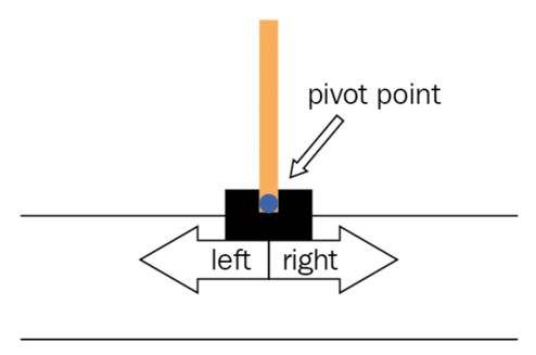
以前我们都是默认在 carpole
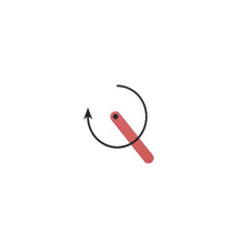
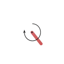
环境中进行实验,这次我们需要在连续动作的环境中,因此选择了Pendulum-v1。简单介绍下环境,详细的会在后续实验中说明。
环境如下。动作是左右摆动,值为一个连续值,范围为:[-2,2]。目标是将杆子立起来,因此立起来的奖励最高。
然后再介绍 DDPG
算法,不过其实我也不太了解算法内容,因为一开始以为就是路径衍生算法 ,后来查了下说是路径衍生算法的一种实现。不过这都不重要,最重要的是理解上一章理论中所说的:在路径衍生策略梯度里面,评论员会直接告诉演员采取什么样的动作才是好的。评论员会直接告诉演员做什么样的动作才可以得到比较大的值。
我们接下来一步步进行解释。
首先,我们 critic 输出是 Q值,即 Q(s,a)。
我们知道, \(Q(s,a) = r +
Q(s',a_{max})\) 。因此,我们从链中,获取一段 \((s_1, a_1, r_1, s_2)\) , 即可计算出 \(Q(s',a_{max})\)
然后用平方差计算损失 critic_loss = mse( \(Q(s',a_{max}) , Q(s,a)\) )
那么,实际上我们不需要收集完完整的链就能直接每步都进行训练 。因为我们只利用到了整个链中的一步数据。
接下来是actor (即下面的策略π), actor
实际上更简单,因为能直接获得Q值,直接全部Q加起来就是总奖励了。
总奖励 R = critic(s, π(s))
因此,actor_loss = -critic(s, π(s))
不过这里有注意的一点,首先我们定义 θ 是actor网络中的参数,动作 \(a = π(s)\) ,那么我们就会存在如下求导过程:
\[
\frac{∂ \text{actor\_loss} }{∂\theta}=\frac{∂ \text{actor\_loss}
}{∂a}\frac{∂ a}{∂\theta}
\] 即,因为存在 \(∂a/∂θ\)
,我们要求a必须是可导的。
举个例子,以前我们通过策略π生成了一个action_logits,然后对其进行
argmax 或者 Category
等函数采样获得动作,这些动作都是不可导的,因为采样这一过程就是不可导的。
而在Pendulum-v1
环境中,动作是连续的,直接由策略π生成出来的的一个值,用tahn激活函数限制在[-2,2]之间,即可拿来当作动作,因此是可导的。
因此DDPG更适合在连续动作的环境下,而非离散动作环境中。
当我们需要减少actor_loss = -critic(s, π(s))
的时候,我们会通过梯度调整动作 \(a =
π(s)\)
,比如减少a能降低loss,由于a只是策略的输出,因此梯度会继续流到策略π的网络中,策略π就会调整自身参数,达到减少a这目的(a是连续值)。这即是评论员评估动作的好坏后给予演员如何做出更好动作的修改方向 。即所谓的。评论员会直接告诉演员做什么样的动作才可以得到比较大的值。
知道以上内容后,我们设计我们的程序如下:
每步收集数据 (s,a,r,s_next,done),收集足够的数据存在buffer中。
从buffer中随机采样batch_size个数据
使用(s,a,r,s_next,done) 中的 s,计算出 actor
的损失 :
actor_loss = Q.mean() = -critic(s, π(s).mean())
使用 s_next 计算出下一动作 a_next = π(s_next)
,然后利用奖励r 计算目标值
y = r + critic(s_next,a_next)
利用 s,a ,计算出我们的当前Q值 :critic(s,a)
用平方差计算 critic 的
loss :critic_loss = mse( critic(s,a) , y)
更新网络
由于 critic
实际上就是DQN中的网络,因此我们也会使用目标网络的方式来减小 y
的波动。即我们用目标网络来计算目标y。
首先,a_next = target_actor(s_next),然后
y = r + target_critic(s_next,a_next)
计算出我们的当前Q值 :critic(s,a)
用平方差计算 critic 的
loss :critic_loss = mse( critic(s,a) , y)
1.3 DDPG算法,Carpole 环境
刚才1.2中我们讲过DDPG并不适合离散的环境,因为离散动作通过采样获得,因此不可导。
这里先说一种失败的方法。起码我没成功
在离散中,该如何成功 反向传播计算 critic(s, π(s)) 呢, 我们给 π(s)
加上一层伪装 : π(s)=[4,123] , get_action (π(s)) =[0,1]
。
get_action内部流程如下:
先计算出 π(s)=[4,123]
然后根据 arg_max 获得 [0,1]
结果 result = [0,1] + π(s) - π(s).detach
由于 [0,1] 和 - π(s).detach
都没有梯度,因此loss计算的梯度沿着π(s)流了回去。而在正向传播中我们仍然获得动作[0,1]
我通过该方法设计出来了网络,但是实验效果非常差,因此谨在此提一下。
那么我们可以转换一个思路,动作不可导,但是动作的分布可导啊。我们actor输出的不就是动作的分布吗。
首先我们设计critic,现在我们不是计算Q值,而是价值V,V=critic(s,d),这里d是一个动作分布。可以简单理解为,提供状态s和动作分布d,critic评估这个状态s值多少价值。
我们知道 \(V = r + γ * V_{next}\)
,因此我们的目标就是 y= r + γ * critic(s_next, d_next),
而我们当前的价值则是 critic(s, d)
。最后我们就能用平方差计算我们的 critic_loss:
critic_loss = MSE(y, critic(s, d))
其实我们这里也能发现,分布d取代了原本动作a的位置,因此我们收集数据的时候,不再是(s,a,r,s'),而是(s,
d, r, s')。和之前一样我们计算critic_loss只需要单步数据中的 s、r、s'
即可,因此也不需要收集完整个episode的数据再训练。
和之前一样,actor也非常简单,总奖励
R = critic(s, actor(s) ).mean() ,因此
actor_loss = -R。(这里 d=actor(s) )。
actor_loss的计算中,我们也仅用到了单步数据中的s,因此也是每步都能更新。
已知以上后,我们能写出程序流程
收集足够的数据,存到buffer中
从buffer中采样batch_size个数据
计算 actor_loss = -critic(s, actor(s) ).mean()
计算下一状态的分布 d_next = actor(s_next) ,计算目标值
y= r + γ * critic(s_next, d_next) ,计算当前价值
critic(s, d) 。
计算 critic_loss = MSE(y, critic(s, d))
更新网络
跟之前,一样,我们也使用了目标网络的方式
首先,d_next = target_actor(s_next),然后
y = r + target_critic(s_next,d_next)
计算出我们的当前Q值 :critic(s,a)
用平方差计算 critic 的
loss :critic_loss = mse( critic(s,a) , y)
2. 优势演员-评论员算法 (A2C)
2.1 环境介绍
我们和之前策略梯度一样,使用的环境是CartPole-v1。也同样是为了方便区分与之前有什么不同。
状态空间:[ 小车位置,小车速度,杆子的角度,杆子的角速度
],4个连续值
动作空间: [左,右],2个离散值
接下来我们创建环境并设置需要的超参数,以及创建我们的 agent 和
data_buffer:
1
2
3
4
5
6
7
8
9
max_steps = 500 n_episodes = 1000 env = gym.make('CartPole-v1' ) state_dim = env.observation_space.shape[0 ] action_dim = env.action_space.n agent = A2CAgent(state_dim, action_dim) data_buffer1 = DataBuffer(max_steps)
2.2 agent 介绍
agent 代码如下。(agent的update函数放在后面讲)
1
2
3
4
5
6
7
8
9
10
11
12
13
14
15
16
17
18
19
20
21
22
23
24
25
26
27
28
29
30
31
32
33
34
35
36
37
38
39
40
class A2CAgent : def __init__ (self, state_dim, action_dim, lr=3e-4 , gamma=0.99 ): self .gamma = gamma self .device = torch.device('cuda' if torch.cuda.is_available() else 'cpu' ) self .actor = Actor(state_dim, action_dim).to(self .device) self .critic = Critic(state_dim, action_dim).to(self .device) self .actor_opt = optim.Adam(self .actor.parameters(), lr=lr) self .critic_opt = optim.Adam(self .critic.parameters(), lr=lr) self .grad_norm_ema = None self .grad_ema_beta = 0.99 def sample_action (self,state ): state = torch.Tensor(state).unsqueeze(0 ).to(self .device) with torch.no_grad(): action_logits = self .actor(state) dist = Categorical(logits=action_logits) action = dist.sample() action = action.cpu().item() return action def state_dict (self ): return { 'actor' : self .actor.state_dict(), 'critic' : self .critic.state_dict(), 'actor_opt' : self .actor_opt.state_dict(), 'critic_opt' : self .critic_opt.state_dict(), } def load_state_dict (self, state_dict ): self .actor.load_state_dict(state_dict['actor' ]) self .critic.load_state_dict(state_dict['critic' ]) self .actor_opt.load_state_dict(state_dict['actor_opt' ]) self .critic_opt.load_state_dict(state_dict['critic_opt' ])
其中actor和critic的网络结构如下
1
2
3
4
5
6
7
8
9
10
11
12
13
14
15
16
17
18
19
20
21
22
23
24
25
26
27
28
29
30
31
32
33
34
35
36
37
38
39
40
41
import torchimport torch.nn as nnimport torch.nn.functional as Fclass Actor (nn.Module): def __init__ (self, n_states, n_actions, hidden_dim = 256 , init_w=3e-3 ): super (Actor, self ).__init__() self .linear1 = nn.Linear(n_states, hidden_dim) self .linear2 = nn.Linear(hidden_dim, hidden_dim) self .linear3 = nn.Linear(hidden_dim, n_actions) self .linear3.weight.data.uniform_(-init_w, init_w) self .linear3.bias.data.uniform_(-init_w, init_w) def forward (self, x ): x = F.relu(self .linear1(x)) x = F.relu(self .linear2(x)) x = self .linear3(x) return x class Critic (nn.Module): def __init__ (self, n_states, n_actions, hidden_dim=256 , init_w=3e-3 ): super (Critic, self ).__init__() self .linear1 = nn.Linear(n_states, hidden_dim) self .linear2 = nn.Linear(hidden_dim, hidden_dim) self .linear3 = nn.Linear(hidden_dim, 1 ) self .linear3.weight.data.uniform_(-init_w, init_w) self .linear3.bias.data.uniform_(-init_w, init_w) def forward (self, state ): x = F.relu(self .linear1(state)) x = F.relu(self .linear2(x)) x = self .linear3(x) return x
2.3 训练流程
根据我们前面的理论部分,我们A2C中需要收集一整条链的数据,然后再开始训练。
1
2
3
4
5
6
7
8
9
10
11
12
13
14
15
16
17
18
for episode in range (n_episodes): state, _ = env.reset() data_buffer1.clean() episode_reward = collect_data(state,max_steps,env,data_buffer1,agent) agent.train_step(data_buffer1) if (episode + 1 ) % 40 == 0 : print (f"回合:{episode+1 } ,奖励:{episode_reward:.2 f} " ) if (episode+1 )%200 ==0 : torch.save(agent.state_dict(), f"A2C_{episode+1 } .pth" ) print (f"Policy saved to A2C_{episode+1 } .pth" )
2.4 收集数据
收集数据的函数,以及我们的数据存储buffer
1
2
3
4
5
6
7
8
9
10
11
12
13
14
15
16
17
18
19
20
21
22
23
24
25
26
27
28
29
30
31
32
33
34
35
36
37
38
39
40
41
42
43
44
45
46
47
48
49
50
51
import randomfrom collections import dequeclass DataBuffer : def __init__ (self, capacity ): self .buffer = deque(maxlen=capacity) self .device = torch.device('cuda' if torch.cuda.is_available() else 'cpu' ) def push (self, s, a, r, s_next, done ): self .buffer.append((s, a, r, s_next, done)) def fetch_data (self ): batch = list (self .buffer)[:len (self .buffer)] s, a, r, s_next, done = zip (*batch) return ( torch.tensor(np.array(s)).to(self .device), torch.tensor(a).to(self .device), torch.tensor(r).to(self .device), torch.tensor(np.array(s_next)).to(self .device), torch.tensor(done, dtype=torch.int64).to(self .device), ) def clean (self ): self .buffer.clear() def __len__ (self ): return len (self .buffer) def collect_data (init_state,max_steps,env,data_buffer,agent:A2CAgent ): state=init_state episode_reward = 0 for step in range (max_steps): state_tensor = torch.FloatTensor(state).unsqueeze(0 ) action = agent.sample_action(state_tensor) next_state, reward, terminated, truncated, _ = env.step(action) done = terminated or truncated data_buffer.push(state,action,reward,next_state,done) episode_reward += reward state = next_state if done: break return episode_reward
2.5 agent训练
根据我们之前的理论部分,一步步求出 actor_loss 和
critic_loss,然后反向传播即可
1
2
3
4
5
6
7
8
9
10
11
12
13
14
15
16
17
18
19
20
21
22
23
24
25
26
27
28
29
30
31
32
33
34
35
36
37
38
39
40
41
42
43
44
45
46
47
48
49
50
51
52
53
54
55
56
57
58
59
60
61
62
63
64
65
66
67
68
69
class A2CAgent : ... def compute_returns (self, rewards, dones ): returns = [] R = 0 for i in reversed (range (len (rewards))): if dones[i]: R = 0 R = rewards[i] + self .gamma * R returns.insert(0 , R) return torch.tensor(returns, dtype=torch.float32).to(self .device) def compute_advantages (self, returns, values ): advantages = returns - values advantages = (advantages - advantages.mean()) / (advantages.std() + 1e-8 ) return advantages def train_step (self, data_buffer:DataBuffer ): states, actions, rewards,s_next, dones = data_buffer.fetch_data() action_logits = self .actor(states) values = self .critic(states) returns = self .compute_returns(rewards, dones) advantages = self .compute_advantages(returns, values.detach()) dist = Categorical(logits=action_logits) log_probs = dist.log_prob(actions) actor_loss = -(log_probs * advantages.detach()).mean() values=values.squeeze(1 ) critic_loss = F.mse_loss(values, returns) def clip (parameters ): total_norm = torch.nn.utils.clip_grad_norm_(parameters, float ('inf' )).item() if self .grad_norm_ema is None : self .grad_norm_ema = total_norm else : self .grad_norm_ema = self .grad_ema_beta * self .grad_norm_ema + (1 - self .grad_ema_beta) * total_norm adaptive_max_norm = max (2.0 * self .grad_norm_ema, 1.0 ) torch.nn.utils.clip_grad_norm_(parameters, adaptive_max_norm) self .actor.zero_grad() actor_loss.backward() clip(self .actor.parameters()) self .actor_opt.step() self .critic.zero_grad() critic_loss.backward() clip(self .critic.parameters()) self .critic_opt.step()
2.6 训练及结果
1
2
3
4
5
6
7
8
9
10
11
12
13
14
15
16
17
18
19
20
21
22
23
24
25
26
27
28
29
30
31
32
33
34
35
36
37
38
39
40
41
42
43
44
45
46
47
device = torch.device("cuda" if torch.cuda.is_available() else "cpu" ) def load_policy (model_path ): state_dim = 4 action_dim = 2 agent = A2CAgent(state_dim, action_dim) agent.load_state_dict(torch.load(model_path)) agent.actor.eval () return agent def render_policy (agent:A2CAgent, episodes=5 ): env = gym.make("CartPole-v1" , render_mode="human" ) for ep in range (episodes): state, _ = env.reset() done = False total_reward = 0 while not done: state_tensor = torch.as_tensor(state, dtype=torch.float32, device=device) with torch.no_grad(): probs = agent.actor(state_tensor) action = torch.argmax(probs).item() state, reward, terminated, truncated, _ = env.step(action) done = terminated or truncated total_reward += reward print (f"Episode {ep} , Total Reward: {total_reward} " ) env.close() if __name__ == "__main__" : print ("开始训练 A2C 智能体(路径衍生策略梯度)..." ) print ("=" * 60 ) train() agent = load_policy("A2C_1000.pth" ) render_policy(agent)
3. DDPG Pendulum-v1环境
3.1 环境介绍
我们使用连续动作的环境Pendulum-v1。
状态空间:[cosθ, sinθ, θ_{dot]} ,3个连续值。其中
θ_dot(角速度),θ_dot ∈ [-8,
8],表示摆转动的速度。
动作空间: 动作是 一个 连续值,action ∈ [-2,
2]。这是施加在摆上的 力矩(torque)
-2:向一个方向最大用力(比如顺时针)
+2:反方向最大用力(逆时针)
0:不施加力
目标:让摆保持在竖直向上(θ =
0)。同时:角速度尽量小,动作(力矩)尽量小(节省能量)。
每一步 reward 大概是:\(reward = -(θ^2 +
0.1 * θ_{dot}^2 + 0.001 * action^2)\)
惩罚:
接下来我们创建环境并设置需要的超参数,以及创建我们的 agent 和
data_buffer:
1
2
3
4
5
6
7
8
9
10
max_steps = 500 n_episodes = 1000 env = gym.make('Pendulum-v1' ) state_dim = env.observation_space.shape[0 ] action_dim = env.action_space.shape[0 ] agent = Agent(state_dim, action_dim) data_buffer = DataBuffer(1000 ) ou_noise = OUNoise(env.action_space)
3.2 agent 介绍
首先是 actor 和 critic。
我们知道动作是一个范围在 [-2, 2] 的连续值,而tanh的输出范围在 [-1, 1]
,因此刚好actor的输出结果乘以2就能覆盖我们的动作范围。
1
2
3
4
5
6
7
8
9
10
11
12
13
14
15
16
17
18
19
20
21
22
23
24
25
26
27
28
29
30
31
32
33
34
35
36
37
38
39
40
41
42
import torchimport torch.nn as nnimport torch.nn.functional as Fclass Actor (nn.Module): def __init__ (self, n_states, n_actions, hidden_dim = 256 , init_w=3e-3 ): super (Actor, self ).__init__() self .linear1 = nn.Linear(n_states, hidden_dim) self .linear2 = nn.Linear(hidden_dim, hidden_dim) self .linear3 = nn.Linear(hidden_dim, n_actions) self .linear3.weight.data.uniform_(-init_w, init_w) self .linear3.bias.data.uniform_(-init_w, init_w) def forward (self, x ): x = F.relu(self .linear1(x)) x = F.relu(self .linear2(x)) x = torch.tanh(self .linear3(x)) return x class Critic (nn.Module): def __init__ (self, n_states, n_actions, hidden_dim=256 , init_w=3e-3 ): super (Critic, self ).__init__() self .linear1 = nn.Linear(n_states + n_actions, hidden_dim) self .linear2 = nn.Linear(hidden_dim, hidden_dim) self .linear3 = nn.Linear(hidden_dim, 1 ) self .linear3.weight.data.uniform_(-init_w, init_w) self .linear3.bias.data.uniform_(-init_w, init_w) def forward (self, state, action ): x = torch.cat([state, action], 1 ) x = F.relu(self .linear1(x)) x = F.relu(self .linear2(x)) x = self .linear3(x) return x
然后是我们的agent。这里我们的目标网络采用的是软更新的方式(参考原书作者代码的使用,
),因此先设置更新所需参数 self.tau 。
1
2
3
4
5
6
7
8
9
10
11
12
13
14
15
16
17
18
19
20
21
22
23
24
25
26
27
28
29
30
31
32
33
34
35
36
37
38
39
40
41
42
43
44
45
46
47
48
import torch.optim as optimclass Agent : def __init__ (self, state_dim, action_dim, lr=3e-4 , gamma=0.99 ): self .device = torch.device('cuda' if torch.cuda.is_available() else 'cpu' ) self .actor = Actor(state_dim,action_dim).to(self .device) self .target_actor = Actor(state_dim,action_dim).to(self .device) for target_param, param in zip (self .target_actor.parameters(), self .actor.parameters()): target_param.data.copy_(param.data) self .critic = Critic(state_dim,action_dim).to(self .device) self .target_critic = Critic(state_dim,action_dim).to(self .device) for target_param, param in zip (self .target_critic.parameters(), self .critic.parameters()): target_param.data.copy_(param.data) self .gamma = gamma self .lr = lr self .actor_opt=optim.Adam(self .actor.parameters(),lr=self .lr) self .critic_opt=optim.Adam(self .critic.parameters(),lr=self .lr) self .tau = 1e-2 def sample_action (self,state ): state=torch.FloatTensor(state).unsqueeze(0 ).to(self .device) action = self .actor(state) return 2 *action.detach().cpu().numpy()[0 ,0 ] def sample_action_in_text (self,state ): state=torch.FloatTensor(state).unsqueeze(0 ).to(self .device) action = self .actor(state) return 2 *action.detach().cpu().numpy()[0 ] def state_dict (self ): return { 'actor' : self .actor.state_dict(), 'critic' : self .critic.state_dict(), 'actor_opt' : self .actor_opt.state_dict(), 'critic_opt' : self .critic_opt.state_dict(), } def load_state_dict (self, state_dict ): self .actor.load_state_dict(state_dict['actor' ]) self .critic.load_state_dict(state_dict['critic' ]) self .actor_opt.load_state_dict(state_dict['actor_opt' ]) self .critic_opt.load_state_dict(state_dict['critic_opt' ])
3.3 训练流程
根据我们理论中所说的,不需要完整收集一个episode的轨迹链,只要buffer中有足够数据采样出batch_size条数据即可。因此可以每步更新。(也不用像A2C中顺序,或者说打乱更有利于训练critic)
1
2
3
4
5
6
7
8
9
10
11
12
13
14
15
16
17
18
19
20
21
22
23
24
25
26
27
28
29
30
31
32
for episode in range (n_episodes): state, _ = env.reset() episode_reward = 0 ou_noise.reset() for step in range (max_steps): action = agent.sample_action(state) action = ou_noise.get_action(action, step + 1 ) next_state, reward, terminated, truncated, _ = env.step(action) done = terminated or truncated data_buffer.push(state, action, reward, next_state, done) episode_reward += reward state = next_state if done: break agent.update(data_buffer) if (episode+1 )%40 == 0 : print (f"回合:{episode+1 } ,奖励:{episode_reward:.2 f} " ) if (episode+1 )%200 ==0 : torch.save(agent.state_dict(), f"Pendulum-v1_{episode+1 } .pth" ) print (f"Policy saved to Pendulum-v1_{episode+1 } .pth" )
可以注意到我们训练中给动作添加了噪音
action = ou_noise.get_action(action, step + 1)
ou_noise的代码如下(直接把原作者的拿过来用了,仅理解为给动作添加随机性即可,因为我们critic需要更多样的(s,a,s_next)
数据组来训练):
1
2
3
4
5
6
7
8
9
10
11
12
13
14
15
16
17
18
19
20
21
22
23
24
25
class OUNoise (object ): '''Ornstein–Uhlenbeck噪声 ''' def __init__ (self, action_space, mu=0.0 , theta=0.15 , max_sigma=0.3 , min_sigma=0.3 , decay_period=100000 ): self .mu = mu self .theta = theta self .sigma = max_sigma self .max_sigma = max_sigma self .min_sigma = min_sigma self .decay_period = decay_period self .n_actions = action_space.shape[0 ] self .low = action_space.low self .high = action_space.high self .reset() def reset (self ): self .obs = np.ones(self .n_actions) * self .mu def evolve_obs (self ): x = self .obs dx = self .theta * (self .mu - x) + self .sigma * np.random.randn(self .n_actions) self .obs = x + dx return self .obs def get_action (self, action, t=0 ): ou_obs = self .evolve_obs() self .sigma = self .max_sigma - (self .max_sigma - self .min_sigma) * min (1.0 , t / self .decay_period) return np.clip(action + ou_obs, self .low, self .high)
buffer代码如下
1
2
3
4
5
6
7
8
9
10
11
12
13
14
15
16
17
18
19
20
21
22
23
24
25
26
27
28
29
30
31
import randomfrom collections import dequeimport numpy as npclass DataBuffer : def __init__ (self, capacity ): self .buffer = deque(maxlen=capacity) self .device = torch.device('cuda' if torch.cuda.is_available() else 'cpu' ) def push (self, s, a, r, s_next, done ): self .buffer.append((s, a, r, s_next, done)) def fetch_data_random (self, batch_size ): batch = random.sample(self .buffer, batch_size) s, a, r, s_next, done = zip (*batch) return ( torch.tensor(np.array(s), dtype=torch.float32).to(self .device), torch.tensor(np.array(a), dtype=torch.float32).to(self .device), torch.tensor(r, dtype=torch.float32).to(self .device), torch.tensor(np.array(s_next), dtype=torch.float32).to(self .device), torch.tensor(done, dtype=torch.float32).to(self .device), ) def length (self ): return len (self .buffer) def clean (self ): self .buffer.clear() def __len__ (self ): return len (self .buffer)
3.4 agent训练
计算 actor_loss 和 critic_loss
部分已经在一开始的理论中讲过了。我们这里说下
目标网络的软更新部分。相比我们一开始学的,每C轮更新一次目标网络(硬更新),在每一步中小幅度更新目标网络效果更好、更稳定。主要在于硬更新在跳变的瞬间,critic的学习目标突然发生改变,可能引起训练震荡,而且我们也不知道C该设置多少合适。而软更新中,我每次只更新目标网络非常少的部分,使目标网络做指数移动平均,比硬更新的突变更平滑,tau
足够小时反而比硬更新更稳定。
1
2
3
4
5
6
7
8
9
10
11
12
13
14
15
16
17
18
19
20
21
22
23
24
25
26
27
28
29
30
31
32
33
34
35
36
37
38
39
40
41
42
43
44
class Agent : ... def update (self,data_buffer: DataBuffer ): if data_buffer.length() < 64 : return states, actions, rewards, s_next, dones = data_buffer.fetch_data_random(64 ) q_values = self .critic(states,self .actor(states)) actor_loss = - q_values.mean() a_next = self .target_actor(s_next) q_value_next = self .target_critic(s_next,a_next) rewards = rewards.unsqueeze(1 ) dones = dones.unsqueeze(1 ) target_values = (rewards+(1.0 -dones) *self .gamma*q_value_next).detach() actual_values = self .critic(states,actions) critic_loss = nn.MSELoss()(actual_values,target_values) self .actor.zero_grad() actor_loss.backward() self .actor_opt.step() self .critic.zero_grad() critic_loss.backward() self .critic_opt.step() for target_param, param in zip (self .target_critic.parameters(), self .critic.parameters()): target_param.data.copy_( target_param.data * (1.0 - self .tau) + param.data * self .tau ) for target_param, param in zip (self .target_actor.parameters(), self .actor.parameters()): target_param.data.copy_( target_param.data * (1.0 - self .tau) + param.data * self .tau )
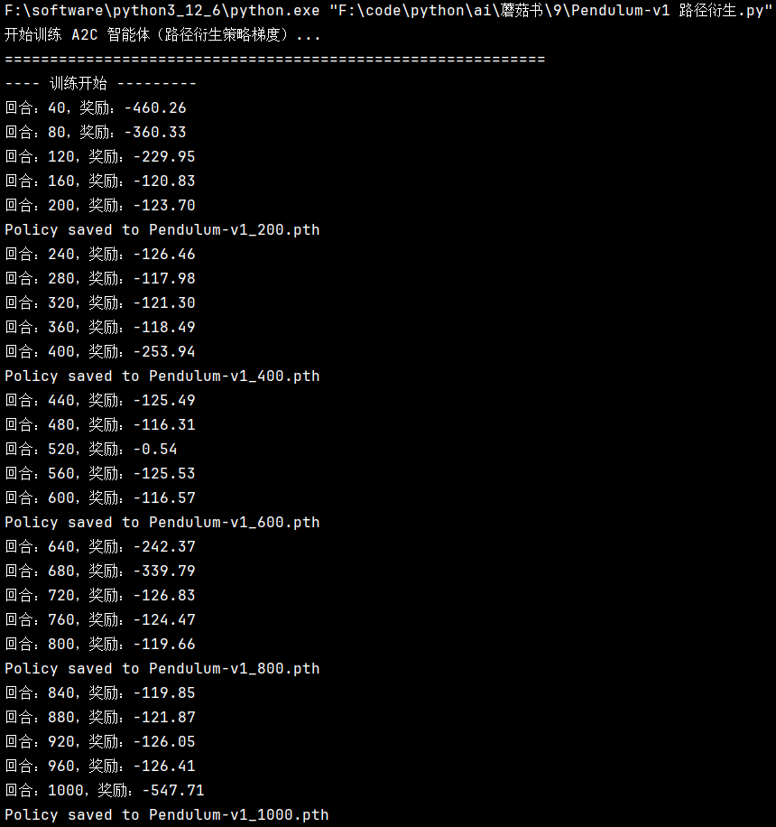
3.6 训练及结果
1
2
3
4
5
6
7
8
9
10
11
12
13
14
15
16
17
18
19
20
21
22
23
24
25
26
27
28
29
30
31
32
33
34
35
36
37
38
39
40
41
42
43
44
45
46
47
48
49
device = torch.device("cuda" if torch.cuda.is_available() else "cpu" ) def load_policy (model_path ): state_dim = 3 action_dim = 1 agent = Agent(state_dim, action_dim) agent.load_state_dict(torch.load(model_path)) agent.actor.eval () return agent def render_policy (agent:Agent, episodes=5 ): env = gym.make('Pendulum-v1' , render_mode="human" ) for ep in range (episodes): state, _ = env.reset() done = False total_reward = 0 while not done: with torch.no_grad(): action = agent.sample_action_in_text(state) state, reward, terminated, truncated, _ = env.step(action) done = terminated or truncated total_reward += reward print (f"Episode {ep} , Total Reward: {total_reward} " ) env.close() if __name__ == "__main__" : print ("开始训练 A2C 智能体(路径衍生策略梯度)..." ) print ("=" * 60 ) agent = load_policy("Pendulum-v1_600.pth" ) render_policy(agent)
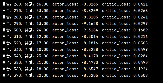
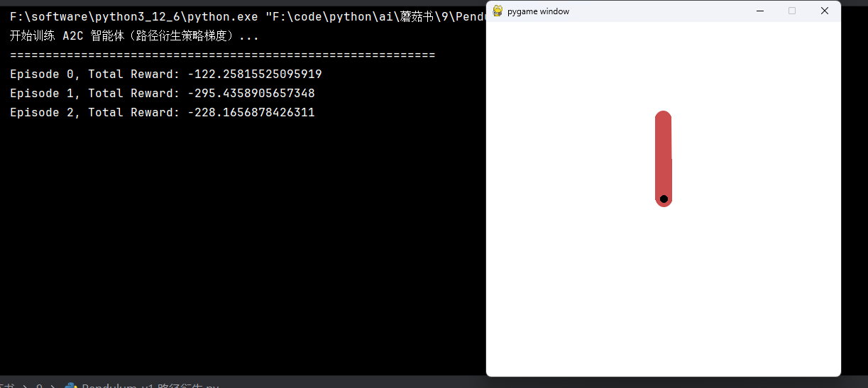
每次都能立起来
4. DDPG Carpole环境
和之前理论中说的那样,DDPG只能处理能求导的actor输出,那么我们对分布求导,不再对动作求导,就能应用DDPG算法了。
4.1 环境设置
创建环境并设置需要的超参数,以及创建我们的 agent 和 data_buffer:
1
2
3
4
5
6
7
8
9
10
max_steps = 500 n_episodes = 1000 env = gym.make('CartPole-v1' ) state_dim = env.observation_space.shape[0 ] action_dim = env.action_space.n agent = Agent(state_dim, action_dim) data_buffer = DataBuffer(1000 )
4.2 agent介绍
还是先看 actor 和 critic。能看到,Actor的最后一层
x = F.softmax(self.linear3(x),dim=-1)
输出直接是概率分布。
1
2
3
4
5
6
7
8
9
10
11
12
13
14
15
16
17
18
19
20
21
22
23
24
25
26
27
28
29
30
31
32
33
34
35
36
37
38
39
40
41
42
import torchimport torch.nn as nnimport torch.nn.functional as Fclass Actor (nn.Module): def __init__ (self, n_states, n_actions, hidden_dim = 256 , init_w=3e-3 ): super (Actor, self ).__init__() self .linear1 = nn.Linear(n_states, hidden_dim) self .linear2 = nn.Linear(hidden_dim, hidden_dim) self .linear3 = nn.Linear(hidden_dim, n_actions) self .linear3.weight.data.uniform_(-init_w, init_w) self .linear3.bias.data.uniform_(-init_w, init_w) def forward (self, x ): x = F.relu(self .linear1(x)) x = F.relu(self .linear2(x)) x = F.softmax(self .linear3(x),dim=-1 ) return x class Critic (nn.Module): def __init__ (self, n_states, n_actions, hidden_dim=256 , init_w=3e-3 ): super (Critic, self ).__init__() self .linear1 = nn.Linear(n_states + n_actions, hidden_dim) self .linear2 = nn.Linear(hidden_dim, hidden_dim) self .linear3 = nn.Linear(hidden_dim, 1 ) self .linear3.weight.data.uniform_(-init_w, init_w) self .linear3.bias.data.uniform_(-init_w, init_w) def forward (self, state, action ): x = torch.cat([state, action], 1 ) x = F.relu(self .linear1(x)) x = F.relu(self .linear2(x)) x = self .linear3(x) return x
然后是我们的agent。之前我们说过,我们的存储的数据不再是
(s,a,r,s',done) 而是
(s,d ,r,s',done)。因此下面sample_action函数的输出中,我们不仅要返回动作a,也还要返回分布
action_prob 。
1
2
3
4
5
6
7
8
9
10
11
12
13
14
15
16
17
18
19
20
21
22
23
24
25
26
27
28
29
30
31
32
33
34
35
36
37
38
39
40
41
42
43
44
45
46
47
48
49
50
51
52
53
54
55
56
from torch.distributions import Categoricalimport torch.optim as optimclass Agent : def __init__ (self, state_dim, action_dim, lr=3e-4 , gamma=0.99 ): self .device = torch.device('cuda' if torch.cuda.is_available() else 'cpu' ) self .actor = Actor(state_dim,action_dim).to(self .device) self .target_actor = Actor(state_dim,action_dim).to(self .device) for target_param, param in zip (self .target_actor.parameters(), self .actor.parameters()): target_param.data.copy_(param.data) self .critic = Critic(state_dim,action_dim).to(self .device) self .target_critic = Critic(state_dim,action_dim).to(self .device) for target_param, param in zip (self .target_critic.parameters(), self .critic.parameters()): target_param.data.copy_(param.data) self .gamma = gamma self .lr = lr self .actor_opt=optim.Adam(self .actor.parameters(),lr=self .lr) self .critic_opt=optim.Adam(self .critic.parameters(),lr=self .lr) self .device = torch.device('cuda' if torch.cuda.is_available() else 'cpu' ) self .tau = 1e-2 self .grad_norm_ema = None self .grad_ema_beta = 0.99 def sample_action (self,state,env,step ): state = torch.Tensor(state).unsqueeze(0 ).to(self .device) with torch.no_grad(): action_prob = self .actor(state) dist = Categorical(probs=action_prob) action = dist.sample() action = action.cpu().item() return action, action_prob.detach().cpu() def state_dict (self ): return { 'actor' : self .actor.state_dict(), 'target_actor' : self .target_actor.state_dict(), 'critic' : self .critic.state_dict(), 'target_critic' : self .target_critic.state_dict(), 'actor_opt' : self .actor_opt.state_dict(), 'critic_opt' : self .critic_opt.state_dict(), } def load_state_dict (self, state_dict ): self .actor.load_state_dict(state_dict['actor' ]) self .target_actor.load_state_dict(state_dict['target_actor' ]) self .critic.load_state_dict(state_dict['critic' ]) self .target_critic.load_state_dict(state_dict['target_critic' ]) self .actor_opt.load_state_dict(state_dict['actor_opt' ]) self .critic_opt.load_state_dict(state_dict['critic_opt' ])
4.3 训练流程
和上一节DDPG的类似,不过我们这里不仅返回了动作,还有分布。以及buffer中存储的是分布。
1
2
3
4
5
6
7
8
9
10
11
12
13
14
15
16
17
18
19
20
21
22
23
24
25
26
27
28
29
30
for episode in range (n_episodes): state, _ = env.reset() episode_reward = 0 for step in range (max_steps): action,action_prob = agent.sample_action(state,env,step) next_state, reward, terminated, truncated, _ = env.step(action) done = terminated or truncated data_buffer.push(state, action_prob, reward, next_state, done) episode_reward += reward state = next_state if done: break agent.update(data_buffer,300 ) if (episode + 1 ) % 40 == 0 : print (f"回合:{episode+1 } ,奖励:{episode_reward:.2 f} " ) if (episode+1 )%200 ==0 : torch.save(agent.state_dict(), f"DDPG_distribute_{episode+1 } .pth" ) print (f"Policy saved to DDPG_distribute_{episode+1 } .pth" )
4.4 agen训练更新
按照之前理论说的,计算 actor_loss 和 critic_loss。然后更新
1
2
3
4
5
6
7
8
9
10
11
12
13
14
15
16
17
18
19
20
21
22
23
24
25
26
27
28
29
30
31
32
33
34
35
36
37
38
39
40
41
42
43
44
45
46
47
48
49
50
51
52
53
54
55
56
57
58
59
60
61
62
class Agent : def update (self,data_buffer: DataBuffer,batch_size ): if data_buffer.length() < batch_size: return states, actions_prob, rewards, s_next, dones = data_buffer.fetch_data_random(batch_size) V = self .critic(states,self .actor(states)) actor_loss = - V.mean() d_next = self .target_actor(s_next) V_next = self .target_critic(s_next,d_next) rewards = rewards.unsqueeze(1 ) dones = dones.unsqueeze(1 ) actions_prob = actions_prob.squeeze(1 ) target_values = (rewards+(1.0 -dones) *self .gamma*V_next).detach() actual_values = self .critic(states,actions_prob) critic_loss = nn.MSELoss()(actual_values,target_values) def clip (parameters ): total_norm = torch.nn.utils.clip_grad_norm_(parameters, float ('inf' )).item() if self .grad_norm_ema is None : self .grad_norm_ema = total_norm else : self .grad_norm_ema = self .grad_ema_beta * self .grad_norm_ema + (1 - self .grad_ema_beta) * total_norm adaptive_max_norm = max (2.0 * self .grad_norm_ema, 1.0 ) torch.nn.utils.clip_grad_norm_(parameters, adaptive_max_norm) self .actor.zero_grad() actor_loss.backward() clip(self .actor.parameters()) self .actor_opt.step() self .critic.zero_grad() critic_loss.backward() clip(self .critic.parameters()) self .critic_opt.step() for target_param, param in zip (self .target_critic.parameters(), self .critic.parameters()): target_param.data.copy_( target_param.data * (1.0 - self .tau) + param.data * self .tau ) for target_param, param in zip (self .target_actor.parameters(), self .actor.parameters()): target_param.data.copy_( target_param.data * (1.0 - self .tau) + param.data * self .tau )
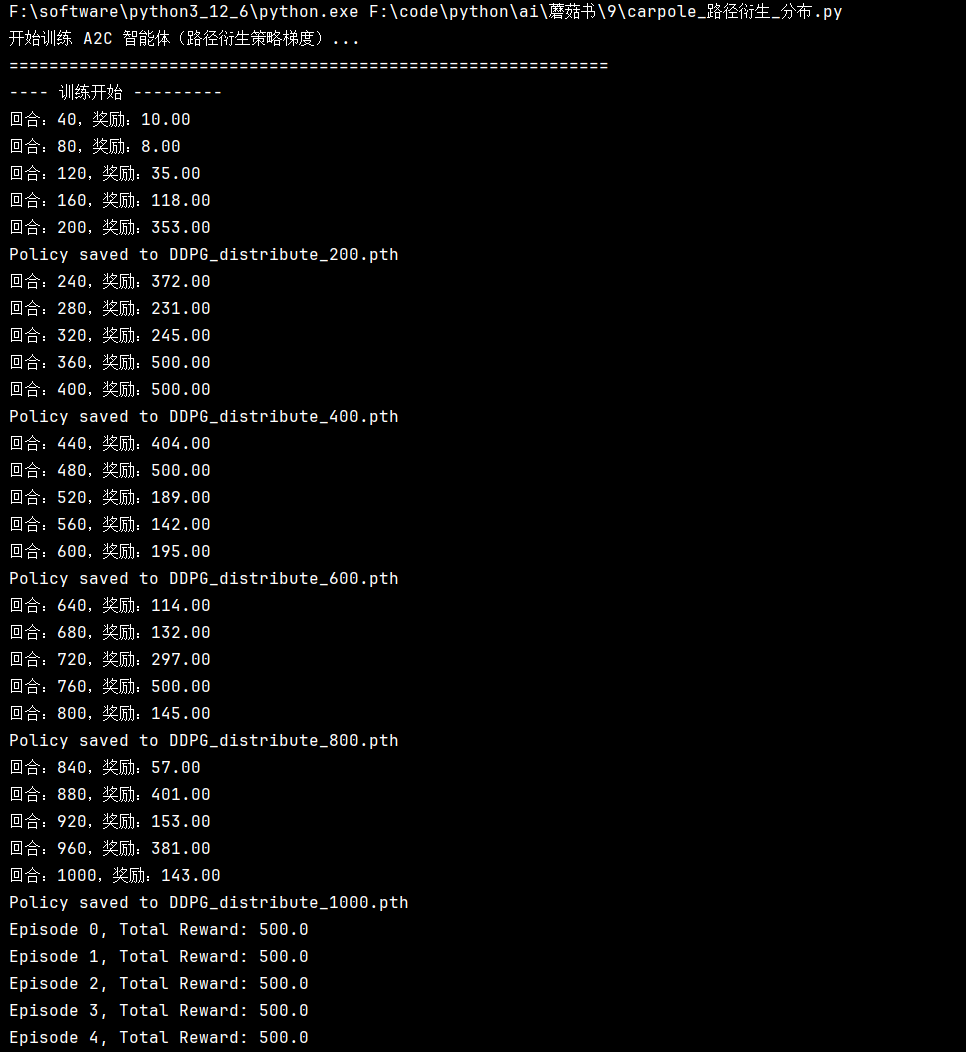
4.5 训练及结果
1
2
3
4
5
6
7
8
9
10
11
12
13
14
15
16
17
18
19
20
21
22
23
24
25
26
27
28
29
30
31
32
33
34
35
36
37
38
39
40
41
42
43
44
45
46
47
48
device = torch.device("cuda" if torch.cuda.is_available() else "cpu" ) def load_policy (model_path ): state_dim = 4 action_dim = 2 agent = Agent(state_dim, action_dim) agent.load_state_dict(torch.load(model_path)) agent.actor.eval () return agent def render_policy (agent:Agent, episodes=5 ): env = gym.make("CartPole-v1" , render_mode="human" ) for ep in range (episodes): state, _ = env.reset() done = False total_reward = 0 while not done: state_tensor = torch.as_tensor(state, dtype=torch.float32, device=device) with torch.no_grad(): probs = agent.actor(state_tensor) action = torch.argmax(probs).item() state, reward, terminated, truncated, _ = env.step(action) done = terminated or truncated total_reward += reward print (f"Episode {ep} , Total Reward: {total_reward} " ) env.close() if __name__ == "__main__" : print ("开始训练 A2C 智能体(路径衍生策略梯度)..." ) print ("=" * 60 ) train() agent = load_policy("DDPG_distribute_600.pth" ) render_policy(agent)
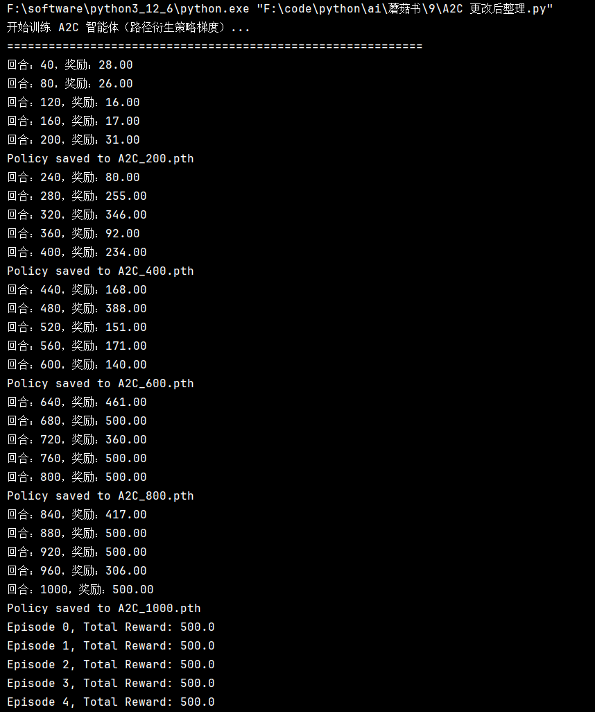
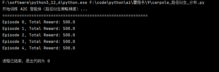
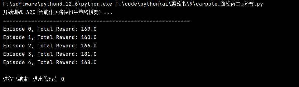
事实上从400轮开始就非常稳定。。
agent = load_policy("DDPG_distribute_400.pth")
但是800轮开始又退化了,不知道为啥